The fastest introduction to machine learning 🧠
A.I is a hot topic nowadays. The goal of this post is to explain as simply as possible the idea behind every known algorithm of machine learning. By using an example I want to make things really clear, and I’ll try to use less math as possibile. I provide also a pdf version of this post. Enjoy!
Disclaimer: for the experiments I used a modified version of Tsoding Daily’s code, which is really clean and easy to understand.
The premise⌗
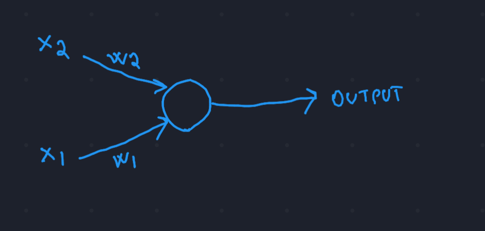
This is a neuron. Our brain is full of them, the more neurons (and connections between them) you have, the more “computational” power you have as a human being. Our intelligence is mainly determined by the number of connections that our brain creates over time.
- x1, x2 \(\rightarrow\) inputs of the neuron, they are bio-electrical impulses that are coming from other connected neurons.
- w1, w2 \(\rightarrow\) weights of each input, they represent “how thick” the connection is, so “how much” of the original input actually passes through the connection.
- output \(\rightarrow\) the impulse that the neuron produces and sends to other connected neurons.
 Computer scientists during the last 30/40 years tried to model something like this using a computer, and right now
they are creating huge brains that are just made of billions of connections between theese really simple neurons.
Computer scientists during the last 30/40 years tried to model something like this using a computer, and right now
they are creating huge brains that are just made of billions of connections between theese really simple neurons.
The goal⌗
The goal of this post is to teach you how one neuron works and how it can learn to recognize really simple patterns, for example the AND gate. For those of you that are not into computer science, what I am refering to is this:
\begin{align} x1=0,x2=0 \rightarrow y = 0 \\ x1=1,x2=0 \rightarrow y = 0 \\ x1=0,x2=1 \rightarrow y = 0 \\ x1=1,x2=1 \rightarrow y = 1 \end{align}
Training the neuron means teaching him how to find the optimal values of w1 and w2 so that it can use them to produce (on a given input of for example \(x1=0\) \(x2=1\)) an output that is as close as possible to the expected output (\(0\) in this case)!
The formula of the neuron⌗
But what does the neuron exactly?
The formula that is “embedded” inside the neuron is the following:
\begin{equation} f(\sum_{i=1}^{N}{(x_{i} \times w_{i}}) + b) = output \end{equation}
where:
- \(N\) is the number of input connections of the neuron (2 in our case);
- \(w_{i}\) are the weights of the connections;
- \(x_{i}\) are the inputs;
- \(f\) is the activation function: it “compresses” the final output of the neuron to make it fit in the \([0,1]\) range. This is used because we want the neuron to only produce an output value that is between \(0\) and \(1\).
- \(b\) is the bias, a single value that is conventionally used to improve the performance of the model. The neuron will understand itself what is the optimal value for this parameter.
The idea behind gradient descent⌗
Our neuron/model is going to have completely random parameters (\(w1\), \(w2\), \(b\)) at the beginning of the training. So it is almost 100% sure that it is going to produce a wrong output when we submit the inputs for the first time. The cool thing is that we can measure the error that it made and try to minimize it over time.
The main goal of a machine learning algorithm is to minimize the error made by the model.
But how do we measure the error?
The error is going to be represented by a function, usually called cost function or loss function. The most common and simple cost function is the Mean Squared Error:
\begin{equation} MSE = \frac{1}{T} * \sum_{i=1}^{T}{(p - y)^2} \end{equation}
where:
- \(T\) is the number of examples that we provide to the model (in our case, 4 examples);
- \(p\) is the output of the neuron, also called prediction;
- \(y\) is the expected output related to the given input;
Let’s treat the loss function as a mathematical function: let’s suppose that it is represented
by a parabola:
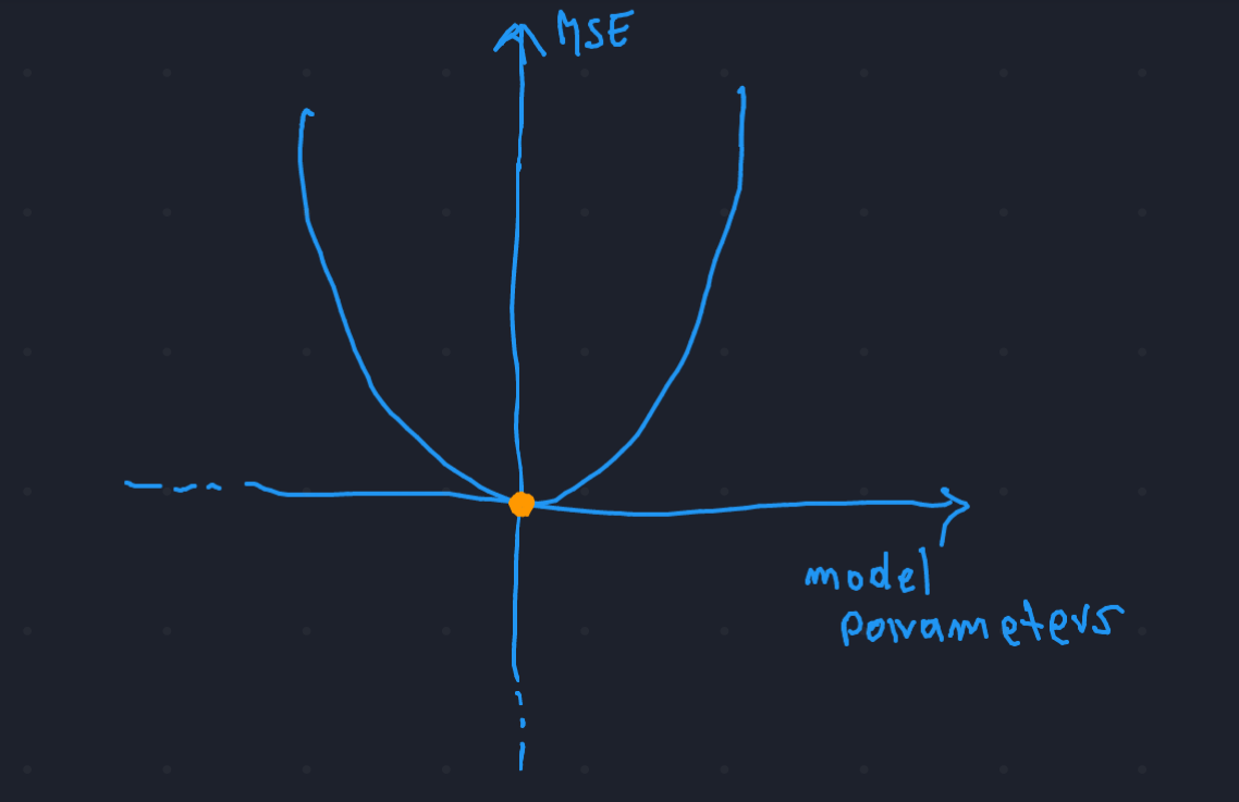 always remember that our goal is to minimize this function: so we have to find a way to tune the parameters of our model (\(w1\),\(w2\),\(b\)) to make the function reach the yellow point!
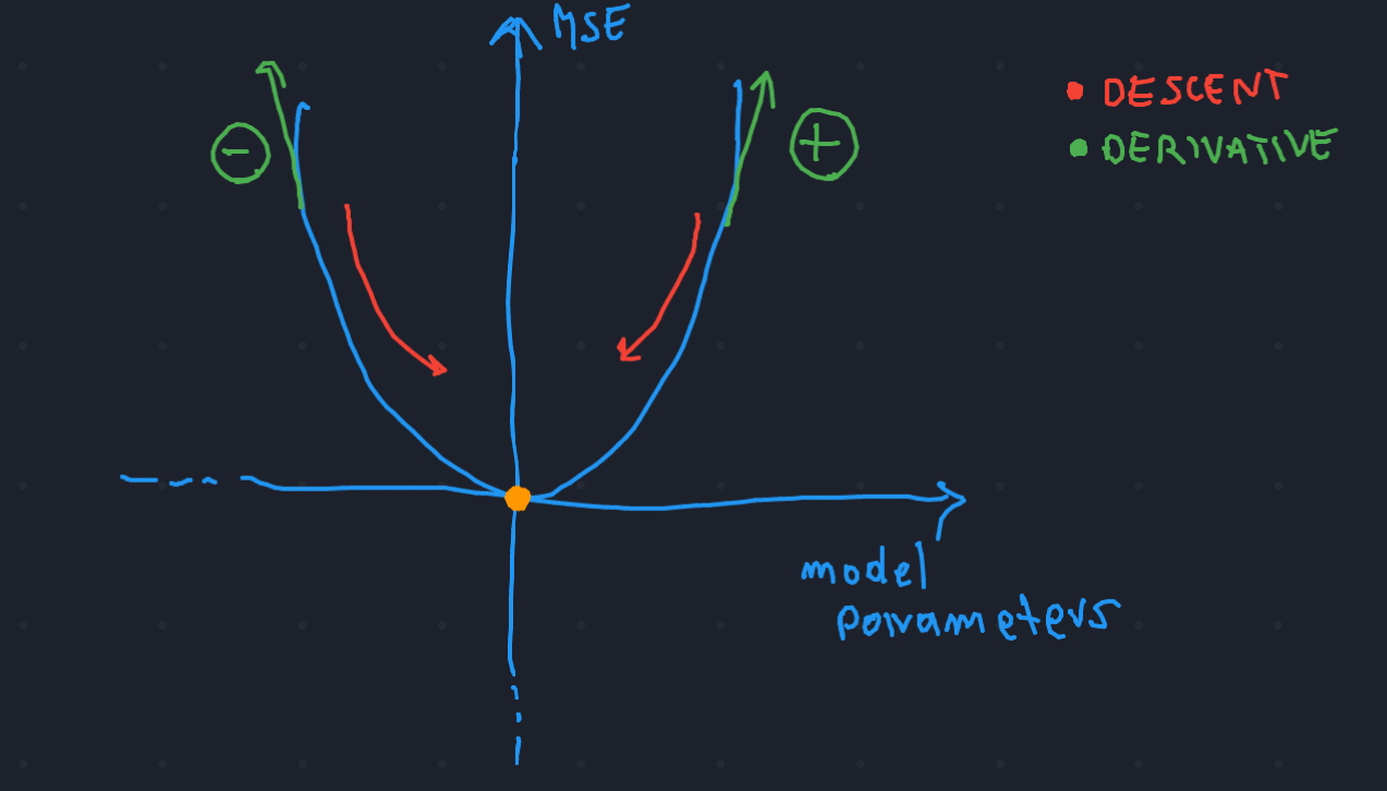
Well, it doesn’t look that hard: if the function is currently growing, that we move our parameters to the left a little bit, if it is decreasing then we move them to the right!
But how do we know if the function is growing/decreasing?
I am sure that you remember from high school that the only way to know if a function is decreasing/increasing is to calculate the derivative of the function in that point! The idea is that we always want to move on the opposite direction of the derivative!
Gradient descent⌗
I think that now you are ready to get in touch for the first time with the formula of gradient descent:
\begin{array}{lcl} w_{i} = w_{i} + \Delta w_{i} \\ \Delta w_{i} = -\epsilon*E'(w_{i}) \\ \end{array}
where:
- \(E\) is the cost function (Mean Squared Error in our case);
- \(\epsilon\) is the learning rate, it represents of how much we want to move towards the minimum (in other words, how big is the step).
If we have multiple parameters (like in our case, where we have 3 parameters) we have to use the above formula for each one of them! (In other words, we want to “correct” each parameter based on the error that we saw in the last iteration, trying to have a smaller error the next time that we compute the output with the neuron).
\begin{array}{lcl} w_{1} = w_{1} + \Delta w_{1} \\ w_{2} = w_{2} + \Delta w_{2} \\ b = b + \Delta b \\ \end{array}
If we repeat this process many times our model will find the minimum of the cost function, and that is a good point to stop the training and start using the neural network!
Finite difference⌗
There is only one problem that we have now.
We don’t really know how the derivative of the loss function looks like, the parabola was just an example to understand the idea of gradient descent. For the purpose of this post, we are going to use a trick that is really good for understanding the general mechanism, but it’s not actually used in the real world.
Let’s go back again to high school and write the definition of derivative, also called finite difference:
\begin{equation} \lim_{h\to 0} f'(x) = \frac{f(x+h) - f(x)}{h} \end{equation}
where:
- \(f\) is the loss function;
- \(x\) is the parameter that we are tuning (one of \(w_{1}\),\(w_{2}\),\(b\));
if we pick a really small h (for example 0.001) we can make this calculus and aproximate correctly the derivative of our loss function!
C++ Code⌗
Simple declaration of the training data:
static float train_x1[4] {0,0,1,1};
static float train_x2[4] {0,1,0,1};
static float train_y[4]  {0,0,0,1};
In the main we initialize the model with random values:
float w1 = (rand()%10+1);
float w2 = (rand()%10+1);
float b = (rand()%5+1);
After that, we define:
- epocs: the number of times that we are going to loop through the train data, to teach the neuron the given examples (training data).
- h: small value used to compute finite difference;
- rate: learning rate \(\epsilon\);
int epocs = 10*1000;
float h = 0.1;
float rate = 0.1;
Now we go through the epochs and we apply the delta rule to each one of the parameters of the model:
for(int i = 0; i < epocs; i++){
  float dloss1 = (loss(w1+h, w2, b) - loss(w1, w2, b))/h;
  float dloss2 = (loss(w1, w2+h, b) - loss(w1, w2, b))/h;
  float dloss3 = (loss(w1, w2, b+h) - loss(w1, w2, b))/h;
  w1 -= rate*dloss1;
  w2 -= rate*dloss2;
  b -= rate*dloss3;
  cout<<"W1: "<<w1<<" W2: "<<w2<<" B: "<<b<<" C: "<<loss(w1,w2, b)<<endl;
}
Once we finished the training, we use the neuron to check if it learned correctly the examples.
cout<<"0 & 0 = "<<sigf(0.0*w1 + 0.0*w2 +b)<<endl;
cout<<"0 & 1 = "<<sigf(0.0*w1 + 1.0*w2 +b)<<endl;
cout<<"1 & 0 = "<<sigf(1.0*w1 + 0.0*w2 +b)<<endl;
cout<<"1 & 1 = "<<sigf(1.0*w1 + 1.0*w2 +b)<<endl;
return 0;
This is the end of the main program, now let’s define
the loss function and the sigmoid function, that we left
behind.
The sigmoid function looks something like this:
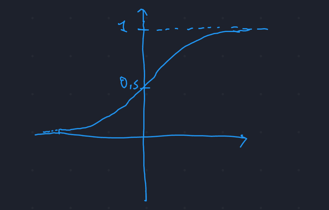 and it is defined as follows, but we don’t really need to
dive into that:
and it is defined as follows, but we don’t really need to
dive into that:
float sigf(float x){
  return 1 / (1 + pow(M_E, -x));
}
Now let’s define the cost function:
float loss(float w1, float w2, float b){
   float result = 0;
   float train_count = 4;
   for(int i = 0; i < train_count; i++){
   float x1 = train_x1[i];
   float x2 = train_x2[i];
   float expected_output = train_y[i];
   float predicted_output = sigf(x1*w1 + x2*w2 + b);
   float mse = pow((expected_output - predicted_output),2); // mean squared error
   result += mse;
   }
   return result / train_count;
}
As you can see we apply and return the Mean Squared Error! If you try this code by yourself, you’ll see that the algorithm drives the cost function to zero, learning the examples really well.
Conclusions⌗
With this post we went through the basics of machine learning. We used the “finite difference trick” with a really simple model to keep things clear, avoiding the backpropagation algorithm (used for models that have multiple layers). With the C++ code, we used a low-level representation to see in practice what we studied before.
I hope that this brief introduction helped some of you in getting in touch with some of the math behind every ML algorithm. If you spot any errors or typos please contact me at matteolugli18@gmail.com. See you soon! Matteo 🐨